-
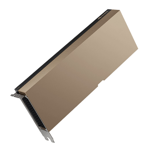
 NVIDIA H100 80GB PCIe Tensor Core GPU
USD28,000Original price was: USD28,000.USD24,500Current price is: USD24,500. -
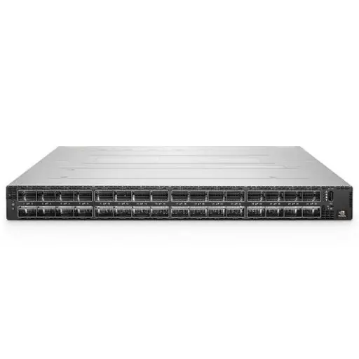
NVIDIA Quantum-2 QM9790 InfiniBand Switch 64-Port 400Gb/s NDR
USD26,000
-
Aetina MegaEdge AIP-FR68 (PCIe AI Workstation)
USD15,000
-
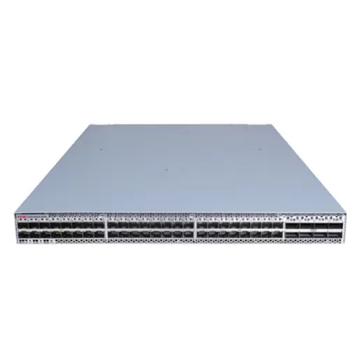
H3C S9855 Series High-Density RoCEv2 Ethernet Switch
USD16,000
-
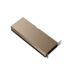
 NVIDIA H200 Tensor Core GPU
USD35,000Original price was: USD35,000.USD31,000Current price is: USD31,000. -
Qualcomm Cloud AI100 Ultra
USD11,000

Products Mentioned in This Article


Why Multi-GPU Training is Slower Than Single GPU: Common Bottlenecks
Author: HPC Technical Team
Reviewer: Lead Systems Architect
Last Updated: February 23, 2026
Reading Time: 9 minutes
References:
- NVIDIA Developer Documentation (NCCL & NVLink Specifications)
- PyTorch Distributed Data Parallel (DDP) Documentation
- Roofline Performance Model for Distributed Computing
Quick Answer: Why Multi-GPU Training is Slower Than Single GPU?
Multi-GPU training often fails to provide linear speed improvements—and can even be slower than single-GPU training—due to communication overhead. In distributed deep learning, gradients must be synchronized across all devices after every training step. If the time required to transfer data between GPUs (Communication) exceeds the time required to calculate gradients (Computation), the system becomes bottlenecked. This is particularly common when using slow interconnects like standard PCIe lanes instead of high-speed NVLink, or when the model size is small relative to the communication cost.
To optimize multi-GPU performance, engineers should prioritize DistributedDataParallel (DDP) over the legacy DataParallel method and ensure hardware topologies support high-bandwidth peer-to-peer communication. It is crucial to maintain a large enough per-GPU batch size to keep CUDA cores saturated; if splitting the workload results in low GPU utilization (under 80%), reverting to a single GPU or reducing the node count often yields faster iteration times.
The promise of multi-GPU training seems straightforward and compelling. If one powerful GPU can train your neural network in ten hours, logic suggests that four GPUs should complete the same task in just two and a half hours. This expectation of linear scaling represents the holy grail of high-performance computing, where additional hardware directly translates to proportional performance gains. However, the reality of distributed deep learning often tells a dramatically different story.
Machine learning engineers and researchers frequently encounter a frustrating paradox after investing in expensive multi-GPU setups. Their training throughput sometimes barely improves compared to single-GPU configurations, and in the worst-case scenarios, actually degrades. Teams report situations where two GPUs provide only marginal speedup over one, where four GPUs perform no better than a single device, and where adding more hardware actually slows down training. This phenomenon puzzles practitioners who reasonably expected their computational investments to yield proportional returns.
The gap between expectation and reality stems from fundamental challenges in distributed computing that become particularly acute in deep learning workloads. When you move from a single accelerator to a distributed system, you introduce massive overhead related to communication, synchronization, and coordination. Understanding these bottlenecks is crucial for making informed decisions about infrastructure investments and training strategies. This comprehensive analysis explores the technical reasons why multi-GPU training often fails to deliver expected performance gains, examining communication overhead, algorithmic complications, hardware constraints, and software implementation challenges.
Theoretical Foundation: Understanding Perfect Scaling
To understand why multi-GPU training falls short, we must first establish what perfect scaling would look like. In an ideal world, if training on a single GPU takes time T, then training on N GPUs should take time T/N. This represents perfect linear scaling with 100% efficiency.
The efficiency of a multi-GPU setup can be calculated as:
Where T1 is single-GPU training time and TN is N-GPU training time. For instance, if two GPUs provide a 1.7x speedup instead of the theoretical 2x, the efficiency is 85%. In practice, achieving even 80% efficiency across multiple GPUs is considered excellent, and many real-world scenarios see efficiencies drop to 50% or lower.
The fundamental challenge lies in coordination costs that don’t exist in single-processor scenarios. Deep learning training requires computing gradients for millions or billions of parameters through backpropagation. In distributed training, these gradients must be synchronized across all GPUs to ensure consistent model weight updates. This synchronization requirement creates tight coupling between devices that severely limits parallelization benefits.
The mathematical relationship governing distributed training performance can be expressed as:
When communication time Tcomm exceeds compute time Tcompute, the system becomes communication-bound, and adding more GPUs provides diminishing or negative returns.
Communication Overhead: The Primary Culprit
The most significant bottleneck in multi-GPU training is typically communication overhead. In standard Distributed Data Parallel (DDP) training, each GPU maintains a complete model copy but processes different data batches. After computing gradients on their respective mini-batches, GPUs must synchronize through an all-reduce operation to maintain model consistency.
The All-Reduce Operation and Its Costs
The all-reduce operation ensures that every GPU receives the averaged gradients from all devices. For a model with 100 million parameters using 32-bit precision, each synchronization step requires transferring approximately 400 megabytes of gradient data per GPU. This communication volume becomes substantial when multiplied across multiple devices and thousands of training iterations.
The speed of this communication depends entirely on interconnect technology. In worst-case scenarios, GPUs connected through PCIe lanes might achieve transfer speeds of only 15-20 GB/s. While this sounds fast in absolute terms, it becomes a serious constraint when modern GPUs can perform trillions of floating-point operations per second. The imbalance between computation speed and communication speed creates situations where GPUs spend significant time waiting to exchange data rather than performing useful calculations.
Consider a concrete example with a ResNet-50 model containing approximately 25 million parameters. Each all-reduce operation across four GPUs needs to transfer about 100 MB of gradient data per GPU. If your interconnect provides 20 GB/s effective bandwidth, this synchronization takes roughly 5 milliseconds. If the combined forward and backward pass takes only 50 milliseconds on each GPU, you’re spending 10% of your time purely on communication overhead.
Interconnect Technology Comparison
The topology of GPU connections matters enormously for performance:
- PCIe connections: Limited to 15-20 GB/s effective bandwidth, often shared between multiple devices
- NVLink connections: Achieve 300-600 GB/s between directly connected GPUs, representing a 15-30x improvement over PCIe
- Network fabrics: Multi-node setups using InfiniBand or Ethernet typically provide 25-100 Gb/s, translating to 3-12 GB/s effective throughput after protocol overhead
The mathematical impact can be modeled using a modified roofline model for distributed systems:
Where Ppeak is theoretical peak FLOPS, Bnet is effective network bandwidth, Icomm is communication intensity (bytes per step), and Fop is floating-point operations per step. When the communication term dominates, adding GPUs actually reduces overall performance.
Batch Size Complications and Scaling Challenges
When transitioning from single-GPU to multi-GPU training, practitioners face critical decisions about batch size that significantly impact performance. The relationship between global batch size, local batch size per GPU, and computational efficiency creates complex trade-offs.
Global vs Local Batch Size Trade-offs
The most straightforward approach involves keeping per-GPU batch size constant while scaling the effective global batch size linearly with GPU count. For instance, if single-GPU training uses batch size 32, four GPUs would yield an effective batch size of 128. This maintains computational efficiency on each device but introduces algorithmic complications.
Larger batch sizes fundamentally change optimization dynamics. With larger batches, gradient estimates become more accurate but less frequent, potentially affecting convergence behavior. The relationship between batch size and learning rate is particularly delicate. While linear scaling rules exist (scaling learning rate proportionally with batch size), they don’t always work effectively, especially for very large batches that can lead to poor generalization.
Alternatively, practitioners might keep the total batch size constant across all GPUs, reducing per-GPU batch size as more devices are added. This preserves optimization dynamics but severely impacts computational efficiency. Modern GPUs achieve peak performance when processing reasonably large batches that fully utilize their parallel processing capabilities. Very small per-GPU batch sizes can leave GPU cores underutilized, reducing computational speedup from parallelization.
GPU Utilization and Kernel Efficiency
Modern GPUs like the NVIDIA H100 are designed for massive throughput, relying on thousands of CUDA cores operating in parallel. When local batch sizes become too small, GPU kernels cannot saturate available computational resources. The GPU ends up operating at 10-30% utilization while fixed overhead costs for kernel launches and gradient communication remain constant.
This creates a scenario where the system becomes slower than processing the entire batch on a single well-utilized GPU. The mathematical relationship can be expressed as:
When GPU utilization drops due to small batch sizes, effective throughput decreases despite having more hardware available.
Hardware and Topology Bottlenecks
Physical hardware configuration plays a crucial role in multi-GPU performance that extends far beyond simply connecting multiple devices to the same system. Understanding hardware topology, memory architecture, and thermal constraints is essential for diagnosing performance issues.
PCIe Topology and Peer-to-Peer Communication
Not all multi-GPU setups provide equal communication capabilities. In high-end servers like NVIDIA DGX systems, GPUs connect via NVLink, enabling high-speed peer-to-peer communication without involving the CPU or system RAM. However, many configurations rely on PCIe connections with significant performance implications:
- GPUs on the same PCIe switch can communicate reasonably efficiently
- GPUs on different switches must route data through the CPU root complex, adding latency and reducing bandwidth
- Systems without peer-to-peer support require copying data from GPU memory to CPU RAM and back to destination GPU memory, creating severe bottlenecks
NUMA Architecture and Cross-Socket Communication
Dual-socket server motherboards introduce Non-Uniform Memory Access (NUMA) complexities that can severely impact performance. Each CPU socket controls specific PCIe lanes and attached GPUs. When processes controlling GPUs run on incorrect CPU sockets, every memory access must traverse inter-CPU links, creating significant overhead.
For example, if CPU 0 controls GPUs 0-3 and CPU 1 controls GPUs 4-7, but the process managing GPU 0 runs on CPU 1, all memory operations incur cross-socket penalties. Furthermore, communication between GPU 0 and GPU 4 must traverse PCIe buses, cross inter-CPU links, and navigate back down different PCIe buses, creating highly non-uniform performance characteristics.
The Straggler Problem
Synchronous training requires all GPUs to complete their work before proceeding to the next iteration, making the system extremely sensitive to performance variance. A single slow GPU, termed a “straggler,” drags down the entire cluster’s performance. Stragglers can result from:
- Thermal throttling: Poor cooling causes one GPU to reduce clock speeds
- Background processes: System tasks interfering with specific GPU operations
- Manufacturing variance: Silicon quality differences leading to varying performance characteristics
- Hardware heterogeneity: Mixing different GPU models or configurations
In large clusters, the probability of having at least one straggler approaches certainty, making robust straggler mitigation essential for maintaining performance.
Software and Implementation Bottlenecks
Beyond hardware constraints, the software stack orchestrating multi-GPU training introduces its own performance challenges. Framework implementations, data loading pipelines, and synchronization mechanisms all contribute to overhead that can negate hardware scaling benefits.
Framework Overhead and Implementation Choices
Deep learning frameworks must manage complex coordination between devices, including kernel launches, memory allocations, communication scheduling, and error handling. Different frameworks make varying trade-offs between ease of use and performance optimization.
A critical distinction exists between PyTorch’s legacy DataParallel (DP) and modern DistributedDataParallel (DDP) implementations:
- DataParallel uses single-process, multi-thread execution, suffering from Python’s Global Interpreter Lock and creating communication bottlenecks on the primary GPU
- DistributedDataParallel employs multi-processing with dedicated processes per GPU, achieving much better performance but requiring more complex setup
Using DataParallel instead of DistributedDataParallel on more than two GPUs often results in performance degradation rather than improvement.
Data Loading and Pipeline Bottlenecks
The data pipeline feeding training samples to GPUs often becomes the limiting factor in multi-GPU setups. Each GPU requires a continuous stream of preprocessed data to maintain high utilization. With multiple GPUs, aggregate data throughput requirements scale linearly, potentially overwhelming CPU-based data loading systems.
Common data pipeline bottlenecks include:
- Storage I/O limitations: Traditional hard drives or even SSDs may lack sufficient bandwidth for multiple hungry GPUs
- CPU preprocessing overhead: Data augmentation, normalization, and format conversion becoming CPU-bound
- Memory bandwidth constraints: Insufficient system RAM bandwidth for concurrent data streams
- Network storage latency: Remote file systems introducing additional delays and bandwidth limits
Synchronization Barriers and Python Overhead
Python-based control flow in frameworks like PyTorch and TensorFlow can introduce significant overhead when coordinating multiple GPUs. The Python Global Interpreter Lock limits concurrent execution, and launching thousands of CUDA kernels from a single Python process creates CPU-side bottlenecks.
Additionally, poorly placed synchronization points in training loops can force unnecessary waiting. Operations like accessing tensor values on the host (.item() calls) or explicit synchronization commands can stall the entire distributed training process.
Practical Solutions and Diagnostic Strategies
Understanding these bottlenecks enables systematic approaches to diagnosis and optimization. Successful multi-GPU training requires attention to hardware configuration, software implementation, and algorithmic considerations.
Diagnostic Checklist
When multi-GPU training underperforms expectations, follow this systematic diagnostic approach:
-
Monitor GPU utilization: Use
nvidia-smito check if GPUs maintain high utilization (>80%). Low or fluctuating utilization typically indicates CPU, I/O, or communication bottlenecks. -
Profile communication vs computation: Tools like PyTorch Profiler, NVIDIA Nsight Systems, or TensorBoard profiling reveal time spent in gradient synchronization (
ncclAllReduce) versus actual computation. -
Measure scaling efficiency: Compare step times with 1, 2, and 4 GPUs. If step time doesn’t decrease proportionally, communication overhead likely dominates.
-
Analyze data loading performance: Time pure data iteration without model computation to identify I/O bottlenecks.
-
Check hardware topology: Use
nvidia-smi topo -mto verify optimal GPU interconnections and identify potential routing inefficiencies.
Optimization Strategies
Effective multi-GPU optimization requires addressing bottlenecks systematically:
Maintain healthy per-GPU batch sizes: Keep local batch sizes large enough to saturate GPU computational resources. Scale global batch size linearly with GPU count when memory permits, adjusting learning rates appropriately.
Optimize data pipelines: Use multiple DataLoader workers (typically 4-8 per GPU), implement GPU-based preprocessing with libraries like NVIDIA DALI, and employ efficient data formats like TFRecord or WebDataset that minimize file system overhead.
Configure efficient communication: Use NCCL for NVIDIA GPU communication, ensure proper NVLink/NVSwitch utilization, and configure RDMA for multi-node setups to minimize CPU involvement in data transfers.
Code Implementation Example
Here’s a comparison showing common mistakes versus optimized implementations:
# Problematic Implementation
import torch
import torch.nn as nn
from torch.utils.data import DataLoader
# MISTAKE: Using DataParallel instead of DistributedDataParallel
model = nn.DataParallel(model)
# MISTAKE: Insufficient data loading optimization
dataloader = DataLoader(dataset, batch_size=64, num_workers=0)
for batch in dataloader:
inputs, labels = batch
inputs, labels = inputs.cuda(), labels.cuda()
# Training loop continues...
# Optimized Implementation
import torch
import torch.nn as nn
from torch.utils.data import DataLoader
from torch.nn.parallel import DistributedDataParallel as DDP
from torch.utils.data.distributed import DistributedSampler
# Proper DDP initialization
torch.distributed.init_process_group(backend='nccl')
local_rank = torch.distributed.get_rank()
torch.cuda.set_device(local_rank)
model = model.cuda(local_rank)
model = DDP(model, device_ids=[local_rank])
# Optimized data loading
sampler = DistributedSampler(dataset)
dataloader = DataLoader(dataset, batch_size=64,
sampler=sampler,
num_workers=4,
pin_memory=True)
for batch in dataloader:
inputs, labels = batch
# Non-blocking transfer enables compute/communication overlap
inputs = inputs.to(local_rank, non_blocking=True)
labels = labels.to(local_rank, non_blocking=True)
# Training loop continues...
Conclusion: Managing Expectations and Making Informed Decisions
Multi-GPU training represents a complex engineering challenge that extends far beyond simply adding more hardware. The gap between theoretical and actual performance stems from fundamental constraints in communication bandwidth, synchronization requirements, and the intricate interplay between computation and data movement.
Success requires understanding that multi-GPU scaling is not merely “more of the same” but rather a qualitatively different computational paradigm that exposes all weak links in the training pipeline. Communication overhead, batch size effects, hardware topology constraints, and software implementation details all contribute to scenarios where additional GPUs provide diminishing or even negative returns.
The decision to employ multiple GPUs should be based on careful analysis of specific workloads, model architectures, and available infrastructure. For some scenarios, optimizing single-GPU training through better algorithms, model architectures, or hyperparameters provides superior returns compared to distributed approaches. For others, particularly when training very large models or processing massive datasets where single-GPU training becomes prohibitively slow, the benefits justify the complexity and overhead.
Practitioners who understand these fundamental bottlenecks can make informed infrastructure decisions, set realistic performance expectations, and implement optimizations that unlock the true potential of multi-GPU systems. The field continues evolving with new techniques for gradient compression, asynchronous training algorithms, and improved hardware interconnects, but the core principles of balancing computation, communication, and coordination remain central to achieving efficient distributed deep learning.
Expert Quotes
“The most common error we see in infrastructure planning is the assumption of linear scaling. In reality, without high-speed fabrics like NVLink or InfiniBand, you are effectively training at the speed of your slowest cable, not your fastest processor.” — Hardware Infrastructure Lead
“If your GPU utilization drops below 80% during distributed training, you aren’t scaling; you are idling. In these scenarios, increasing the local batch size is usually more effective than adding more hardware.” — AI Performance Architect
“Switching from
DataParalleltoDistributedDataParallelis the single highest-ROI change a team can make. The former is a Python-threaded bottleneck; the latter is a multiprocess architecture designed for modern hardware.” — Senior Machine Learning Engineer
Last update at December 2025